Note
Click here to download the full example code
Tutorial for Generative Models of Graphs
Author: Mufei Li, Lingfan Yu, Zheng Zhang
In earlier tutorials we have seen how learned embedding of a graph and/or a node allow applications such as semi-supervised classification for nodes or sentiment analysis. Wouldn’t it be interesting to predict the future evolution of the graph and perform the analysis iteratively?
We will need to generate a variety of graph samples, in other words, we need generative models of graphs. Instead of and/or in addition to learning node and edge features, we want to model the distribution of arbitrary graphs. While general generative models can model the density function explicitly and implicitly and generate samples at once or sequentially, we will only focus on explicit generative models for sequential generation here. Typical applications include drug/material discovery, chemical processes, proteomics, etc.
Introduction
The primitive actions of mutating a graph in DGL are nothing more than add_nodes
and add_edges. That is, if we were to draw a circle of 3 nodes,

we can simply write the code as:
import dgl

g = dgl.DGLGraph()
g.add_nodes(1)              # Add node 0
g.add_nodes(1)              # Add node 1

# Edges in DGLGraph are directed by default.
# For undirected edges, we add edges for both directions.
g.add_edges([1, 0], [0, 1]) # Add edges (1, 0), (0, 1)
g.add_nodes(1)              # Add node 2
g.add_edges([2, 1], [1, 2]) # Add edges (2, 1), (1, 2)
g.add_edges([2, 0], [0, 2]) # Add edges (2, 0), (0, 2)
Real-world graphs are much more complex. There are many families of graphs, with different sizes, topologies, node types, edge types, and the possibility of multigraphs. Besides, a same graph can be generated in many different orders. Regardless, the generative process entails a few steps:
- Encode a changing graph,
- Perform actions stochastically,
- Collect error signals and optimize the model parameters (If we are training)
When it comes to implementation, another important aspect is speed: how do we parallelize the computation given that generating a graph is fundamentally a sequential process?
Note
To be sure, this is not necessarily a hard constraint, one can imagine that subgraphs can be built in parallel and then get assembled. But we will restrict ourselves to the sequential processes for this tutorial.
In tutorial, we will first focus on how to train and generate one graph at a time, exploring parallelism within the graph embedding operation, an essential building block. We will end with a simple optimization that delivers a 2x speedup by batching across graphs.
DGMG: the main flow
We pick DGMG ( Learning Deep Generative Models of Graphs ) as an exercise to implement a graph generative model using DGL, primarily because its algorithmic framework is general but also challenging to parallelize.
Note
While it’s possible for DGMG to handle complex graphs with typed nodes, typed edges and multigraphs, we only present a simplified version of it for generating graph topologies.
DGMG generates a graph by following a state machine, which is basically a two-level loop: generate one node at a time, and connect it to a subset of the existing nodes, one at a time. This is similar to language modeling: the generative process is an iterative one that emits one word/character/sentence at a time, conditioned on the sequence generated so far.
- At each time step, we either
- add a new node to the graph, or
- select two existing nodes and add an edge between them
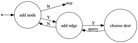
The Python code will look as follows; in fact, this is exactly how inference with DGMG is implemented in DGL:
def forward_inference(self):
    stop = self.add_node_and_update()
    while (not stop) and (self.g.number_of_nodes() < self.v_max + 1):
        num_trials = 0
        to_add_edge = self.add_edge_or_not()
        while to_add_edge and (num_trials < self.g.number_of_nodes() - 1):
            self.choose_dest_and_update()
            num_trials += 1
            to_add_edge = self.add_edge_or_not()
        stop = self.add_node_and_update()

    return self.g
Assume we have a pre-trained model for generating cycles of nodes 10 - 20, let’s see how it generates a cycle on the fly during inference. You can also use the code below for creating animation with your own model.
import torch
import matplotlib.animation as animation
import matplotlib.pyplot as plt
import networkx as nx
from copy import deepcopy

if __name__ == '__main__':
    # pre-trained model saved with path ./model.pth
    model = torch.load('./model.pth')
    model.eval()
    g = model()

    src_list = g.edges()[1]
    dest_list = g.edges()[0]

    evolution = []

    nx_g = nx.Graph()
    evolution.append(deepcopy(nx_g))

    for i in range(0, len(src_list), 2):
        src = src_list[i].item()
        dest = dest_list[i].item()
        if src not in nx_g.nodes():
            nx_g.add_node(src)
            evolution.append(deepcopy(nx_g))
        if dest not in nx_g.nodes():
            nx_g.add_node(dest)
            evolution.append(deepcopy(nx_g))
        nx_g.add_edges_from([(src, dest), (dest, src)])
        evolution.append(deepcopy(nx_g))

    def animate(i):
        ax.cla()
        g_t = evolution[i]
        nx.draw_circular(g_t, with_labels=True, ax=ax,
                         node_color=['#FEBD69'] * g_t.number_of_nodes())

    fig, ax = plt.subplots()
    ani = animation.FuncAnimation(fig, animate,
                                  frames=len(evolution),
                                  interval=600)

DGMG: optimization objective
Similar to language modeling, DGMG trains the model with behavior cloning, or teacher forcing. Let’s assume for each graph there exists a sequence of oracle actions \(a_{1},\cdots,a_{T}\) that generates it. What the model does is to follow these actions, compute the joint probabilities of such action sequences, and maximize them.
By chain rule, the probability of taking \(a_{1},\cdots,a_{T}\) is:
The optimization objective is then simply the typical MLE loss:
def forward_train(self, actions):
    """
    - actions: list
        - Contains a_1, ..., a_T described above
    - self.prepare_for_train()
        - Initializes self.action_step to be 0, which will get
          incremented by 1 every time it is called.
        - Initializes objects recording log p(a_t|a_1,...a_{t-1})

    Returns
    -------
    - self.get_log_prob(): log p(a_1, ..., a_T)
    """
    self.prepare_for_train()

    stop = self.add_node_and_update(a=actions[self.action_step])
    while not stop:
        to_add_edge = self.add_edge_or_not(a=actions[self.action_step])
        while to_add_edge:
            self.choose_dest_and_update(a=actions[self.action_step])
            to_add_edge = self.add_edge_or_not(a=actions[self.action_step])
        stop = self.add_node_and_update(a=actions[self.action_step])

    return self.get_log_prob()
The key difference between forward_train and forward_inference is
that the training process takes oracle actions as input, and returns log
probabilities for evaluating the loss.
DGMG: the implementation
The DGMG class
Below one can find the skeleton code for the model. We will gradually fill in the details for each function.
import torch.nn as nn


class DGMGSkeleton(nn.Module):
    def __init__(self, v_max):
        """
        Parameters
        ----------
        v_max: int
            Max number of nodes considered
        """
        super(DGMGSkeleton, self).__init__()

        # Graph configuration
        self.v_max = v_max

    def add_node_and_update(self, a=None):
        """Decide if to add a new node.
        If a new node should be added, update the graph."""
        return NotImplementedError

    def add_edge_or_not(self, a=None):
        """Decide if a new edge should be added."""
        return NotImplementedError

    def choose_dest_and_update(self, a=None):
        """Choose destination and connect it to the latest node.
        Add edges for both directions and update the graph."""
        return NotImplementedError

    def forward_train(self, actions):
        """Forward at training time. It records the probability
        of generating a ground truth graph following the actions."""
        return NotImplementedError

    def forward_inference(self):
        """Forward at inference time.
        It generates graphs on the fly."""
        return NotImplementedError

    def forward(self, actions=None):
        # The graph we will work on
        self.g = dgl.DGLGraph()

        # If there are some features for nodes and edges,
        # zero tensors will be set for those of new nodes and edges.
        self.g.set_n_initializer(dgl.frame.zero_initializer)
        self.g.set_e_initializer(dgl.frame.zero_initializer)

        if self.training:
            return self.forward_train(actions=actions)
        else:
            return self.forward_inference()
Encoding a dynamic graph
All the actions generating a graph are sampled from probability distributions. In order to do that, we must project the structured data, namely the graph, onto an Euclidean space. The challenge is that such process, called embedding, needs to be repeated as the graphs mutate.
Graph Embedding
Let \(G=(V,E)\) be an arbitrary graph. Each node \(v\) has an embedding vector \(\textbf{h}_{v} \in \mathbb{R}^{n}\). Similarly, the graph has an embedding vector \(\textbf{h}_{G} \in \mathbb{R}^{k}\). Typically, \(k > n\) since a graph contains more information than an individual node.
The graph embedding is a weighted sum of node embeddings under a linear transformation:
The first term, \(\text{Sigmoid}(g_m(\textbf{h}_{v}))\), computes a gating function and can be thought as how much the overall graph embedding attends on each node. The second term \(f_{m}:\mathbb{R}^{n}\rightarrow\mathbb{R}^{k}\) maps the node embeddings to the space of graph embeddings.
We implement graph embedding as a GraphEmbed class:
import torch


class GraphEmbed(nn.Module):
    def __init__(self, node_hidden_size):
        super(GraphEmbed, self).__init__()

        # Setting from the paper
        self.graph_hidden_size = 2 * node_hidden_size

        # Embed graphs
        self.node_gating = nn.Sequential(
            nn.Linear(node_hidden_size, 1),
            nn.Sigmoid()
        )
        self.node_to_graph = nn.Linear(node_hidden_size,
                                       self.graph_hidden_size)

    def forward(self, g):
        if g.number_of_nodes() == 0:
            return torch.zeros(1, self.graph_hidden_size)
        else:
            # Node features are stored as hv in ndata.
            hvs = g.ndata['hv']
            return (self.node_gating(hvs) *
                    self.node_to_graph(hvs)).sum(0, keepdim=True)
Update node embeddings via graph propagation
The mechanism of updating node embeddings in DGMG is similar to that for graph convolutional networks. For a node \(v\) in the graph, its neighbor \(u\) sends a message to it with
where \(\textbf{x}_{u,v}\) is the embedding of the edge between \(u\) and \(v\).
After receiving messages from all its neighbors, \(v\) summarizes them with a node activation vector
and use this information to update its own feature:
Performing all the operations above once for all nodes synchronously is called one round of graph propagation. The more rounds of graph propagation we perform, the longer distance messages travel throughout the graph.
With dgl, we implement graph propagation with g.update_all. Note that
the message notation here can be a bit confusing. While the authors refer
to \(\textbf{m}_{u\rightarrow v}\) as messages, our message function
below only passes \(\text{concat}([\textbf{h}_{u}, \textbf{x}_{u, v}])\).
The operation \(\textbf{W}_{m}\text{concat}([\textbf{h}_{v}, \textbf{h}_{u}, \textbf{x}_{u, v}]) + \textbf{b}_{m}\)
is then performed across all edges at once for efficiency consideration.
from functools import partial

class GraphProp(nn.Module):
    def __init__(self, num_prop_rounds, node_hidden_size):
        super(GraphProp, self).__init__()

        self.num_prop_rounds = num_prop_rounds

        # Setting from the paper
        self.node_activation_hidden_size = 2 * node_hidden_size

        message_funcs = []
        node_update_funcs = []
        self.reduce_funcs = []

        for t in range(num_prop_rounds):
            # input being [hv, hu, xuv]
            message_funcs.append(nn.Linear(2 * node_hidden_size + 1,
                                           self.node_activation_hidden_size))

            self.reduce_funcs.append(partial(self.dgmg_reduce, round=t))
            node_update_funcs.append(
                nn.GRUCell(self.node_activation_hidden_size,
                           node_hidden_size))

        self.message_funcs = nn.ModuleList(message_funcs)
        self.node_update_funcs = nn.ModuleList(node_update_funcs)

    def dgmg_msg(self, edges):
        """For an edge u->v, return concat([h_u, x_uv])"""
        return {'m': torch.cat([edges.src['hv'],
                                edges.data['he']],
                               dim=1)}

    def dgmg_reduce(self, nodes, round):
        hv_old = nodes.data['hv']
        m = nodes.mailbox['m']
        message = torch.cat([
            hv_old.unsqueeze(1).expand(-1, m.size(1), -1), m], dim=2)
        node_activation = (self.message_funcs[round](message)).sum(1)

        return {'a': node_activation}

    def forward(self, g):
        if g.number_of_edges() > 0:
            for t in range(self.num_prop_rounds):
                g.update_all(message_func=self.dgmg_msg,
                             reduce_func=self.reduce_funcs[t])
                g.ndata['hv'] = self.node_update_funcs[t](
                     g.ndata['a'], g.ndata['hv'])
Actions
All actions are sampled from distributions parameterized using neural nets and we introduce them in turn.
Action 1: add nodes
Given the graph embedding vector \(\textbf{h}_{G}\), we evaluate
which is then used to parametrize a Bernoulli distribution for deciding whether to add a new node.
If a new node is to be added, we initialize its feature with
where \(\textbf{h}_{\text{init}}\) is a learnable embedding module for untyped nodes.
import torch.nn.functional as F
from torch.distributions import Bernoulli

def bernoulli_action_log_prob(logit, action):
    """Calculate the log p of an action with respect to a Bernoulli
    distribution. Use logit rather than prob for numerical stability."""
    if action == 0:
        return F.logsigmoid(-logit)
    else:
        return F.logsigmoid(logit)

class AddNode(nn.Module):
    def __init__(self, graph_embed_func, node_hidden_size):
        super(AddNode, self).__init__()

        self.graph_op = {'embed': graph_embed_func}

        self.stop = 1
        self.add_node = nn.Linear(graph_embed_func.graph_hidden_size, 1)

        # If to add a node, initialize its hv
        self.node_type_embed = nn.Embedding(1, node_hidden_size)
        self.initialize_hv = nn.Linear(node_hidden_size + \
                                       graph_embed_func.graph_hidden_size,
                                       node_hidden_size)

        self.init_node_activation = torch.zeros(1, 2 * node_hidden_size)

    def _initialize_node_repr(self, g, node_type, graph_embed):
        """Whenver a node is added, initialize its representation."""
        num_nodes = g.number_of_nodes()
        hv_init = self.initialize_hv(
            torch.cat([
                self.node_type_embed(torch.LongTensor([node_type])),
                graph_embed], dim=1))
        g.nodes[num_nodes - 1].data['hv'] = hv_init
        g.nodes[num_nodes - 1].data['a'] = self.init_node_activation

    def prepare_training(self):
        self.log_prob = []

    def forward(self, g, action=None):
        graph_embed = self.graph_op['embed'](g)

        logit = self.add_node(graph_embed)
        prob = torch.sigmoid(logit)

        if not self.training:
            action = Bernoulli(prob).sample().item()
        stop = bool(action == self.stop)

        if not stop:
            g.add_nodes(1)
            self._initialize_node_repr(g, action, graph_embed)

        if self.training:
            sample_log_prob = bernoulli_action_log_prob(logit, action)

            self.log_prob.append(sample_log_prob)

        return stop
Action 2: add edges
Given the graph embedding vector \(\textbf{h}_{G}\) and the node embedding vector \(\textbf{h}_{v}\) for the latest node \(v\), we evaluate
which is then used to parametrize a Bernoulli distribution for deciding whether to add a new edge starting from \(v\).
class AddEdge(nn.Module):
    def __init__(self, graph_embed_func, node_hidden_size):
        super(AddEdge, self).__init__()

        self.graph_op = {'embed': graph_embed_func}
        self.add_edge = nn.Linear(graph_embed_func.graph_hidden_size + \
                                  node_hidden_size, 1)

    def prepare_training(self):
        self.log_prob = []

    def forward(self, g, action=None):
        graph_embed = self.graph_op['embed'](g)
        src_embed = g.nodes[g.number_of_nodes() - 1].data['hv']

        logit = self.add_edge(torch.cat(
            [graph_embed, src_embed], dim=1))
        prob = torch.sigmoid(logit)

        if self.training:
            sample_log_prob = bernoulli_action_log_prob(logit, action)
            self.log_prob.append(sample_log_prob)
        else:
            action = Bernoulli(prob).sample().item()

        to_add_edge = bool(action == 0)
        return to_add_edge
Action 3: choosing destination
When action 2 returns True, we need to choose a destination for the latest node \(v\).
For each possible destination \(u\in\{0, \cdots, v-1\}\), the probability of choosing it is given by
from torch.distributions import Categorical

class ChooseDestAndUpdate(nn.Module):
    def __init__(self, graph_prop_func, node_hidden_size):
        super(ChooseDestAndUpdate, self).__init__()

        self.graph_op = {'prop': graph_prop_func}
        self.choose_dest = nn.Linear(2 * node_hidden_size, 1)

    def _initialize_edge_repr(self, g, src_list, dest_list):
        # For untyped edges, we only add 1 to indicate its existence.
        # For multiple edge types, we can use a one hot representation
        # or an embedding module.
        edge_repr = torch.ones(len(src_list), 1)
        g.edges[src_list, dest_list].data['he'] = edge_repr

    def prepare_training(self):
        self.log_prob = []

    def forward(self, g, dest):
        src = g.number_of_nodes() - 1
        possible_dests = range(src)

        src_embed_expand = g.nodes[src].data['hv'].expand(src, -1)
        possible_dests_embed = g.nodes[possible_dests].data['hv']

        dests_scores = self.choose_dest(
            torch.cat([possible_dests_embed,
                       src_embed_expand], dim=1)).view(1, -1)
        dests_probs = F.softmax(dests_scores, dim=1)

        if not self.training:
            dest = Categorical(dests_probs).sample().item()

        if not g.has_edge_between(src, dest):
            # For undirected graphs, we add edges for both directions
            # so that we can perform graph propagation.
            src_list = [src, dest]
            dest_list = [dest, src]

            g.add_edges(src_list, dest_list)
            self._initialize_edge_repr(g, src_list, dest_list)

            self.graph_op['prop'](g)

        if self.training:
            if dests_probs.nelement() > 1:
                self.log_prob.append(
                    F.log_softmax(dests_scores, dim=1)[:, dest: dest + 1])
Putting it together
We are now ready to have a complete implementation of the model class.
class DGMG(DGMGSkeleton):
    def __init__(self, v_max, node_hidden_size,
                 num_prop_rounds):
        super(DGMG, self).__init__(v_max)

        # Graph embedding module
        self.graph_embed = GraphEmbed(node_hidden_size)

        # Graph propagation module
        self.graph_prop = GraphProp(num_prop_rounds,
                                    node_hidden_size)

        # Actions
        self.add_node_agent = AddNode(
            self.graph_embed, node_hidden_size)
        self.add_edge_agent = AddEdge(
            self.graph_embed, node_hidden_size)
        self.choose_dest_agent = ChooseDestAndUpdate(
            self.graph_prop, node_hidden_size)

        # Forward functions
        self.forward_train = partial(forward_train, self=self)
        self.forward_inference = partial(forward_inference, self=self)

    @property
    def action_step(self):
        old_step_count = self.step_count
        self.step_count += 1

        return old_step_count

    def prepare_for_train(self):
        self.step_count = 0

        self.add_node_agent.prepare_training()
        self.add_edge_agent.prepare_training()
        self.choose_dest_agent.prepare_training()

    def add_node_and_update(self, a=None):
        """Decide if to add a new node.
        If a new node should be added, update the graph."""

        return self.add_node_agent(self.g, a)

    def add_edge_or_not(self, a=None):
        """Decide if a new edge should be added."""

        return self.add_edge_agent(self.g, a)

    def choose_dest_and_update(self, a=None):
        """Choose destination and connect it to the latest node.
        Add edges for both directions and update the graph."""

        self.choose_dest_agent(self.g, a)

    def get_log_prob(self):
        add_node_log_p = torch.cat(self.add_node_agent.log_prob).sum()
        add_edge_log_p = torch.cat(self.add_edge_agent.log_prob).sum()
        choose_dest_log_p = torch.cat(self.choose_dest_agent.log_prob).sum()
        return add_node_log_p + add_edge_log_p + choose_dest_log_p
Below is an animation where a graph is generated on the fly after every 10 batches of training for the first 400 batches. One can see how our model improves over time and begins generating cycles.
For generative models, we can evaluate its performance by checking the percentage of valid graphs among the graphs it generates on the fly.
import torch.utils.model_zoo as model_zoo

# Download a pre-trained model state dict for generating cycles with 10-20 nodes.
state_dict = model_zoo.load_url('https://s3.us-east-2.amazonaws.com/dgl.ai/model/dgmg_cycles-5a0c40be.pth')
model = DGMG(v_max=20, node_hidden_size=16, num_prop_rounds=2)
model.load_state_dict(state_dict)
model.eval()

def is_valid(g):
    # Check if g is a cycle having 10-20 nodes.
    def _get_previous(i, v_max):
        if i == 0:
            return v_max
        else:
            return i - 1

    def _get_next(i, v_max):
        if i == v_max:
            return 0
        else:
            return i + 1

    size = g.number_of_nodes()

    if size < 10 or size > 20:
        return False

    for node in range(size):
        neighbors = g.successors(node)

        if len(neighbors) != 2:
            return False

        if _get_previous(node, size - 1) not in neighbors:
            return False

        if _get_next(node, size - 1) not in neighbors:
            return False

    return True

num_valid = 0
for i in range(100):
    g = model()
    num_valid += is_valid(g)

del model
print('Among 100 graphs generated, {}% are valid.'.format(num_valid))
Out:
Among 100 graphs generated, 97% are valid.
For the complete implementation, see dgl DGMG example.
Batched Graph Generation
Speeding up DGMG is hard since each graph can be generated with a unique sequence of actions. One way to explore parallelism is to adopt asynchronous gradient descent with multiple processes. Each of them works on one graph at a time and the processes are loosely coordinated by a parameter server. This is the approach that the authors adopted and we can also use.
DGL explores parallelism in the message-passing framework, on top of the framework-provided tensor operation. The earlier tutorial already does that in the message propagation and graph embedding phases, but only within one graph. For a batch of graphs, a for loop is then needed:
for g in g_list:
self.graph_prop(g)
We can modify the code to work on a batch of graphs at once by replacing these lines with the following. On CPU with a Mac machine, we instantly enjoy a 6~7x reduction for the graph propagation part.
bg = dgl.batch(g_list)
self.graph_prop(bg)
g_list = dgl.unbatch(bg)
We have already used this trick of calling dgl.batch in the
Tree-LSTM tutorial
, and it is worth explaining one more time why this is so.
By batching many small graphs, DGL internally maintains a large container
graph (BatchedDGLGraph) over which update_all propels message-passing
on all the edges and nodes.
With dgl.batch, we merge g_{1}, ..., g_{N} into one single giant
graph consisting of \(N\) isolated small graphs. For example, if we
have two graphs with adjacency matrices
[0, 1]
[1, 0]

[0, 1, 0]
[1, 0, 0]
[0, 1, 0]
dgl.batch simply gives a graph whose adjacency matrix is
[0, 1, 0, 0, 0]
[1, 0, 0, 0, 0]
[0, 1, 0, 0, 0]
[1, 0, 0, 0, 0]
[0, 1, 0, 0, 0]
In DGL, the message function is defined on the edges, thus batching scales the processing of edge user-defined functions (UDFs) linearly.
The reduce UDFs (i.e dgmg_reduce) works on nodes, and each of them may
have different numbers of incoming edges. Using degree bucketing, DGL
internally groups nodes with the same in-degrees and calls reduce UDF once
for each group. Thus, batching also reduces number of calls to these UDFs.
The modification of the node/edge features of a BatchedDGLGraph object
does not take effect on the features of the original small graphs, so we
need to replace the old graph list with the new graph list
g_list = dgl.unbatch(bg).
The complete code to the batched version can also be found in the example. On our testbed, we get roughly 2x speed up comparing to the previous implementation
Total running time of the script: ( 0 minutes 5.618 seconds)