Writing GNN Modules for Stochastic GNN Training

All GNN modules DGL provides support stochastic GNN training. This tutorial teaches you how to write your own graph neural network module for stochastic GNN training. It assumes that

1. You know how to write GNN modules for full graph training.

2. You know how stochastic GNN training pipeline works.

import dgl
import torch
import numpy as np
from ogb.nodeproppred import DglNodePropPredDataset

dataset = DglNodePropPredDataset('ogbn-arxiv')
device = 'cpu'      # change to 'cuda' for GPU

graph, node_labels = dataset[0]
# Add reverse edges since ogbn-arxiv is unidirectional.
graph = dgl.add_reverse_edges(graph)
graph.ndata['label'] = node_labels[:, 0]
idx_split = dataset.get_idx_split()
train_nids = idx_split['train']
node_features = graph.ndata['feat']

sampler = dgl.dataloading.MultiLayerNeighborSampler([4, 4])
train_dataloader = dgl.dataloading.NodeDataLoader(
    graph, train_nids, sampler,
    batch_size=1024,
    shuffle=True,
    drop_last=False,
    num_workers=0
)

input_nodes, output_nodes, mfgs = next(iter(train_dataloader))

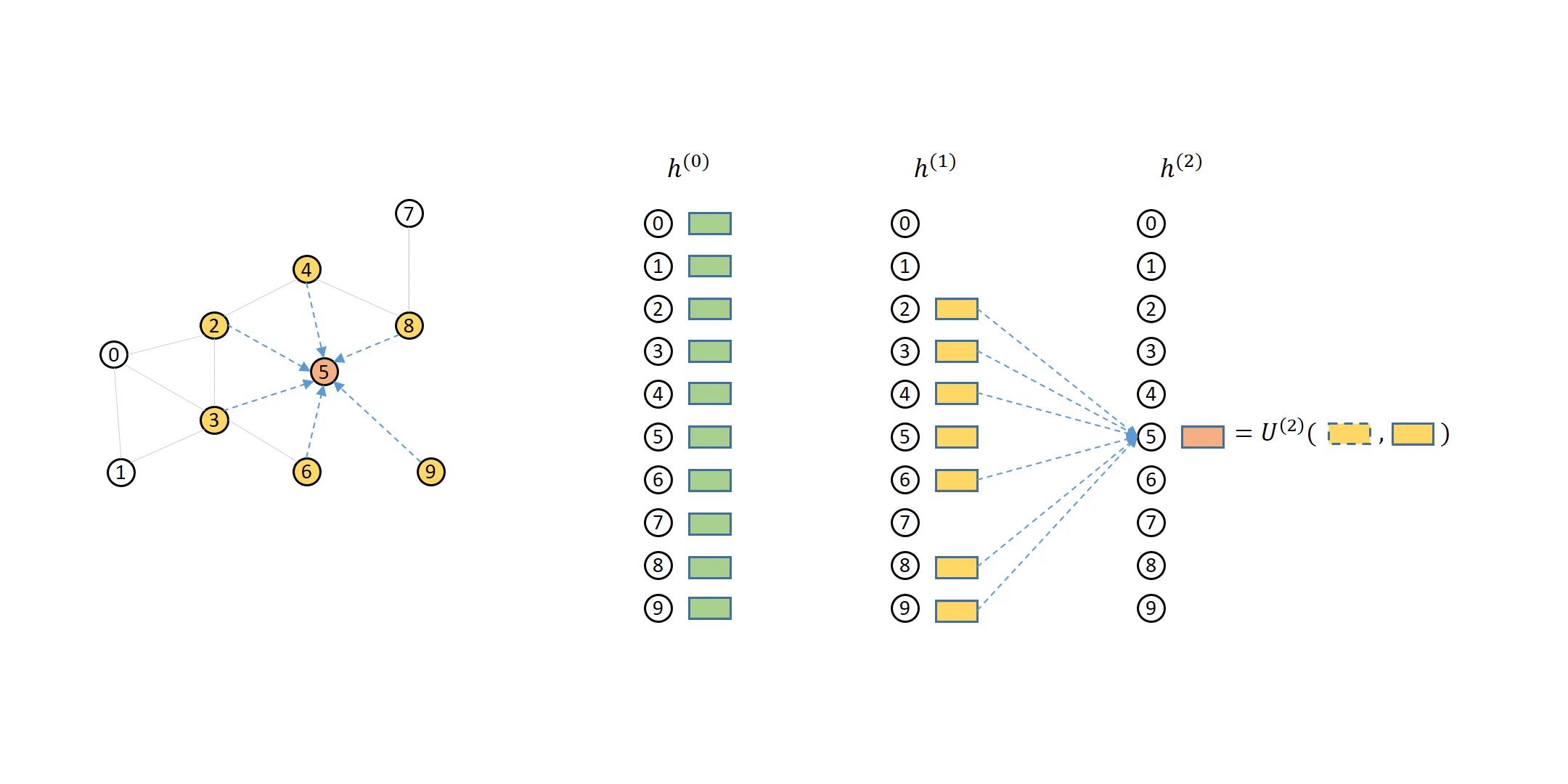
DGL Bipartite Graph Introduction

In the previous tutorials, you have seen the concept message flow graph (MFG), where nodes are divided into two parts. It is a kind of (directional) bipartite graph. This section introduces how you can manipulate (directional) bipartite graphs.

You can access the source node features and destination node features via srcdata and dstdata attributes:

mfg = mfgs[0]
print(mfg.srcdata)
print(mfg.dstdata)

Out:

{'year': tensor([[2017],
        [2016],
        [2006],
        ...,
        [2011],
        [2017],
        [2017]]), 'feat': tensor([[ 0.0346,  0.2829, -0.2166,  ...,  0.2104, -0.2024,  0.0506],
        [ 0.0540,  0.1846, -0.1479,  ...,  0.2975, -0.1924, -0.0469],
        [-0.0821, -0.0278, -0.2437,  ...,  0.3433, -0.0254, -0.0210],
        ...,
        [-0.0717,  0.0101, -0.3163,  ...,  0.2545, -0.0377,  0.0237],
        [ 0.0875,  0.2333, -0.1703,  ...,  0.1147, -0.0790, -0.2870],
        [-0.1286,  0.0212, -0.3371,  ...,  0.1922, -0.1289, -0.1204]]), 'label': tensor([28,  4, 28,  ...,  2,  2,  2]), '_ID': tensor([130088, 139203,  65068,  ...,  66565, 118149, 114642])}
{'year': tensor([[2017],
        [2016],
        [2006],
        ...,
        [2015],
        [2018],
        [2015]]), 'feat': tensor([[ 0.0346,  0.2829, -0.2166,  ...,  0.2104, -0.2024,  0.0506],
        [ 0.0540,  0.1846, -0.1479,  ...,  0.2975, -0.1924, -0.0469],
        [-0.0821, -0.0278, -0.2437,  ...,  0.3433, -0.0254, -0.0210],
        ...,
        [-0.1675,  0.1716, -0.2795,  ...,  0.2186, -0.2493, -0.0766],
        [-0.1006, -0.0501, -0.3241,  ...,  0.3938, -0.0877, -0.0606],
        [-0.1013,  0.0491, -0.1970,  ...,  0.2258, -0.1336, -0.0378]]), 'label': tensor([28,  4, 28,  ...,  2, 39, 39]), '_ID': tensor([130088, 139203,  65068,  ..., 154381, 162076, 104751])}

It also has num_src_nodes and num_dst_nodes functions to query how many source nodes and destination nodes exist in the bipartite graph:

print(mfg.num_src_nodes(), mfg.num_dst_nodes())

Out:

12735 4078

You can assign features to srcdata and dstdata just as what you will do with ndata on the graphs you have seen earlier:

mfg.srcdata['x'] = torch.zeros(mfg.num_src_nodes(), mfg.num_dst_nodes())
dst_feat = mfg.dstdata['feat']

Also, since the bipartite graphs are constructed by DGL, you can retrieve the source node IDs (i.e. those that are required to compute the output) and destination node IDs (i.e. those whose representations the current GNN layer should compute) as follows.

mfg.srcdata[dgl.NID], mfg.dstdata[dgl.NID]

Out:

(tensor([130088, 139203,  65068,  ...,  66565, 118149, 114642]), tensor([130088, 139203,  65068,  ..., 154381, 162076, 104751]))

Writing GNN Modules for Bipartite Graphs for Stochastic Training

Recall that the MFGs yielded by the NodeDataLoader and EdgeDataLoader have the property that the first few source nodes are always identical to the destination nodes:

print(torch.equal(mfg.srcdata[dgl.NID][:mfg.num_dst_nodes()], mfg.dstdata[dgl.NID]))

Out:

True

Suppose you have obtained the source node representations \(h_u^{(l-1)}\):

mfg.srcdata['h'] = torch.randn(mfg.num_src_nodes(), 10)

Recall that DGL provides the update_all interface for expressing how to compute messages and how to aggregate them on the nodes that receive them. This concept naturally applies to bipartite graphs like MFGs – message computation happens on the edges between source and destination nodes of the edges, and message aggregation happens on the destination nodes.

For example, suppose the message function copies the source feature (i.e. \(M^{(l)}\left(h_v^{(l-1)}, h_u^{(l-1)}, e_{u\to v}^{(l-1)}\right) = h_v^{(l-1)}\)), and the reduce function averages the received messages. Performing such message passing computation on a bipartite graph is no different than on a full graph:

import dgl.function as fn

mfg.update_all(message_func=fn.copy_u('h', 'm'), reduce_func=fn.mean('m', 'h'))
m_v = mfg.dstdata['h']
m_v

Out:

tensor([[ 1.1051,  0.5413, -0.1277,  ..., -0.4532, -0.0877,  0.1251],
        [ 0.4618,  0.8092,  0.8738,  ..., -0.7398,  0.0585, -0.5031],
        [-0.7374,  0.4607,  1.1110,  ...,  0.1712, -0.7758, -0.6917],
        ...,
        [ 0.3916,  0.1805, -0.7551,  ..., -0.2750, -0.0501,  0.1933],
        [ 0.8209, -0.7344, -0.8398,  ...,  0.0341, -0.1685,  0.6585],
        [ 0.6547, -0.1451, -0.7135,  ...,  0.6813,  0.7258,  0.3635]])

Putting them together, you can implement a GraphSAGE convolution for training with neighbor sampling as follows (the differences to the full graph counterpart are highlighted with arrows <---)

import torch.nn as nn
import torch.nn.functional as F
import tqdm

class SAGEConv(nn.Module):
    """Graph convolution module used by the GraphSAGE model.

    Parameters
    ----------
    in_feat : int
        Input feature size.
    out_feat : int
        Output feature size.
    """
    def __init__(self, in_feat, out_feat):
        super(SAGEConv, self).__init__()
        # A linear submodule for projecting the input and neighbor feature to the output.
        self.linear = nn.Linear(in_feat * 2, out_feat)

    def forward(self, g, h):
        """Forward computation

        Parameters
        ----------
        g : Graph
            The input MFG.
        h : (Tensor, Tensor)
            The feature of source nodes and destination nodes as a pair of Tensors.
        """
        with g.local_scope():
            h_src, h_dst = h
            g.srcdata['h'] = h_src                        # <---
            g.dstdata['h'] = h_dst                        # <---
            # update_all is a message passing API.
            g.update_all(fn.copy_u('h', 'm'), fn.mean('m', 'h_N'))
            h_N = g.dstdata['h_N']
            h_total = torch.cat([h_dst, h_N], dim=1)      # <---
            return self.linear(h_total)

class Model(nn.Module):
    def __init__(self, in_feats, h_feats, num_classes):
        super(Model, self).__init__()
        self.conv1 = SAGEConv(in_feats, h_feats)
        self.conv2 = SAGEConv(h_feats, num_classes)

    def forward(self, mfgs, x):
        h_dst = x[:mfgs[0].num_dst_nodes()]
        h = self.conv1(mfgs[0], (x, h_dst))
        h = F.relu(h)
        h_dst = h[:mfgs[1].num_dst_nodes()]
        h = self.conv2(mfgs[1], (h, h_dst))
        return h

sampler = dgl.dataloading.MultiLayerNeighborSampler([4, 4])
train_dataloader = dgl.dataloading.NodeDataLoader(
    graph, train_nids, sampler,
    device=device,
    batch_size=1024,
    shuffle=True,
    drop_last=False,
    num_workers=0
)
model = Model(graph.ndata['feat'].shape[1], 128, dataset.num_classes).to(device)

with tqdm.tqdm(train_dataloader) as tq:
    for step, (input_nodes, output_nodes, mfgs) in enumerate(tq):
        inputs = mfgs[0].srcdata['feat']
        labels = mfgs[-1].dstdata['label']
        predictions = model(mfgs, inputs)

Out:

  0%|          | 0/89 [00:00<?, ?it/s]
  7%|6         | 6/89 [00:00<00:01, 55.81it/s]
 13%|#3        | 12/89 [00:00<00:01, 56.37it/s]
 20%|##        | 18/89 [00:00<00:01, 56.88it/s]
 27%|##6       | 24/89 [00:00<00:01, 54.51it/s]
 34%|###3      | 30/89 [00:00<00:01, 55.60it/s]
 40%|####      | 36/89 [00:00<00:00, 56.28it/s]
 47%|####7     | 42/89 [00:00<00:00, 56.64it/s]
 54%|#####3    | 48/89 [00:00<00:00, 56.79it/s]
 61%|######    | 54/89 [00:00<00:00, 57.04it/s]
 67%|######7   | 60/89 [00:01<00:00, 57.06it/s]
 74%|#######4  | 66/89 [00:01<00:00, 57.23it/s]
 81%|########  | 72/89 [00:01<00:00, 57.28it/s]
 88%|########7 | 78/89 [00:01<00:00, 57.24it/s]
 94%|#########4| 84/89 [00:01<00:00, 55.29it/s]
100%|##########| 89/89 [00:01<00:00, 56.40it/s]

Both update_all and the functions in nn.functional namespace support MFGs, so you can migrate the code working for small graphs to large graph training with minimal changes introduced above.

Writing GNN Modules for Both Full-graph Training and Stochastic Training

Here is a step-by-step tutorial for writing a GNN module for both full-graph training and stochastic training.

Say you start with a GNN module that works for full-graph training only:

class SAGEConv(nn.Module):
    """Graph convolution module used by the GraphSAGE model.

    Parameters
    ----------
    in_feat : int
        Input feature size.
    out_feat : int
        Output feature size.
    """
    def __init__(self, in_feat, out_feat):
        super().__init__()
        # A linear submodule for projecting the input and neighbor feature to the output.
        self.linear = nn.Linear(in_feat * 2, out_feat)

    def forward(self, g, h):
        """Forward computation

        Parameters
        ----------
        g : Graph
            The input graph.
        h : Tensor
            The input node feature.
        """
        with g.local_scope():
            g.ndata['h'] = h
            # update_all is a message passing API.
            g.update_all(message_func=fn.copy_u('h', 'm'), reduce_func=fn.mean('m', 'h_N'))
            h_N = g.ndata['h_N']
            h_total = torch.cat([h, h_N], dim=1)
            return self.linear(h_total)

First step: Check whether the input feature is a single tensor or a pair of tensors:

if isinstance(h, tuple):
    h_src, h_dst = h
else:
    h_src = h_dst = h

Second step: Replace node features h with h_src or h_dst, and assign the node features to srcdata or dstdata, instead of ndata.

Whether to assign to srcdata or dstdata depends on whether the said feature acts as the features on source nodes or destination nodes of the edges in the message functions (in update_all or apply_edges).

Example 1: For the following update_all statement:

g.ndata['h'] = h
g.update_all(message_func=fn.copy_u('h', 'm'), reduce_func=fn.mean('m', 'h_N'))

The node feature h acts as source node feature because 'h' appeared as source node feature. So you will need to replace h with source feature h_src and assign to srcdata for the version that works with both cases:

g.srcdata['h'] = h_src
g.update_all(message_func=fn.copy_u('h', 'm'), reduce_func=fn.mean('m', 'h_N'))

Example 2: For the following apply_edges statement:

g.ndata['h'] = h
g.apply_edges(fn.u_dot_v('h', 'h', 'score'))

The node feature h acts as both source node feature and destination node feature. So you will assign h_src to srcdata and h_dst to dstdata:

g.srcdata['h'] = h_src
g.dstdata['h'] = h_dst
# The first 'h' corresponds to source feature (u) while the second 'h' corresponds to destination feature (v).
g.apply_edges(fn.u_dot_v('h', 'h', 'score'))

Note

For homogeneous graphs (i.e. graphs with only one node type and one edge type), srcdata and dstdata are aliases of ndata. So you can safely replace ndata with srcdata and dstdata even for full-graph training.

Third step: Replace the ndata for outputs with dstdata.

For example, the following code

# Assume that update_all() function has been called with output node features in `h_N`.
h_N = g.ndata['h_N']
h_total = torch.cat([h, h_N], dim=1)

will change to

h_N = g.dstdata['h_N']
h_total = torch.cat([h_dst, h_N], dim=1)

Putting together, you will change the SAGEConvForBoth module above to something like the following:

class SAGEConvForBoth(nn.Module):
    """Graph convolution module used by the GraphSAGE model.

    Parameters
    ----------
    in_feat : int
        Input feature size.
    out_feat : int
        Output feature size.
    """
    def __init__(self, in_feat, out_feat):
        super().__init__()
        # A linear submodule for projecting the input and neighbor feature to the output.
        self.linear = nn.Linear(in_feat * 2, out_feat)

    def forward(self, g, h):
        """Forward computation

        Parameters
        ----------
        g : Graph
            The input graph.
        h : Tensor or tuple[Tensor, Tensor]
            The input node feature.
        """
        with g.local_scope():
            if isinstance(h, tuple):
                h_src, h_dst = h
            else:
                h_src = h_dst = h

            g.srcdata['h'] = h_src
            # update_all is a message passing API.
            g.update_all(message_func=fn.copy_u('h', 'm'), reduce_func=fn.mean('m', 'h_N'))
            h_N = g.ndata['h_N']
            h_total = torch.cat([h_dst, h_N], dim=1)
            return self.linear(h_total)


# Thumbnail credits: Representation Learning on Networks, Jure Leskovec, WWW 2018
# sphinx_gallery_thumbnail_path = '_static/blitz_3_message_passing.png'