7.1 Data Preprocessing¶

Before launching training jobs, DGL requires the input data to be partitioned and distributed to the target machines. For relatively small graphs, DGL provides a partitioning API partition_graph() that partitions an in-memory DGLGraph object. It supports multiple partitioning algorithms such as random partitioning and Metis. The benefit of Metis partitioning is that it can generate partitions with minimal edge cuts to reduce network communication for distributed training and inference. DGL uses the latest version of Metis with the options optimized for the real-world graphs with power-law distribution. After partitioning, the API constructs the partitioned results in a format that is easy to load during the training. For example,

import dgl

g = ...  # create or load a DGLGraph object
dgl.distributed.partition_graph(g, 'mygraph', 2, 'data_root_dir')

will outputs the following data file.

data_root_dir/
  |-- mygraph.json          # metadata JSON. File name is the given graph name.
  |-- part0/                # data for partition 0
  |  |-- node_feats.dgl     # node features stored in binary format
  |  |-- edge_feats.dgl     # edge features stored in binary format
  |  |-- graph.dgl          # graph structure of this partition stored in binary format
  |
  |-- part1/                # data for partition 1
     |-- node_feats.dgl
     |-- edge_feats.dgl
     |-- graph.dgl

Chapter 7.4 Advanced Graph Partitioning covers more details about the partition format. To distribute the partitions to a cluster, users can either save the data in some shared folder accessible by all machines, or copy the metadata JSON as well as the corresponding partition folder partX to the X^th machine.

Using partition_graph() requires an instance with large enough CPU RAM to hold the entire graph structure and features, which may not be viable for graphs with hundreds of billions of edges or large features. We describe how to use the parallel data preparation pipeline for such cases next.

Parallel Data Preparation Pipeline¶

To handle massive graph data that cannot fit in the CPU RAM of a single machine, DGL utilizes data chunking and parallel processing to reduce memory footprint and running time. The figure below illustrates the pipeline:

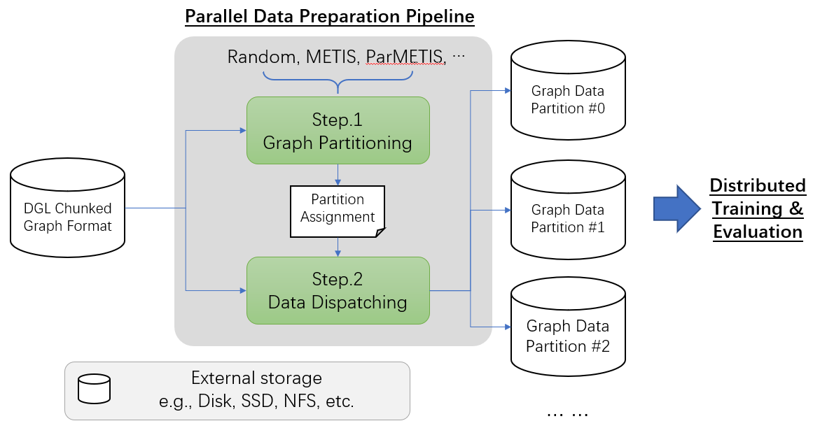
https://data.dgl.ai/asset/image/guide_7_distdataprep.png

The pipeline takes input data stored in Chunked Graph Format and produces and dispatches data partitions to the target machines.
Step.1 Graph Partitioning: It calculates the ownership of each partition and saves the results as a set of files called partition assignment. To speedup the step, some algorithms (e.g., ParMETIS) support parallel computing using multiple machines.
Step.2 Data Dispatching: Given the partition assignment, the step then physically partitions the graph data and dispatches them to the machines user specified. It also converts the graph data into formats that are suitable for distributed training and evaluation.

The whole pipeline is modularized so that each step can be invoked individually. For example, users can replace Step.1 with some custom graph partition algorithm as long as it produces partition assignment files correctly.

Chunked Graph Format¶

To run the pipeline, DGL requires the input graph to be stored in multiple data chunks. Each data chunk is the unit of data preprocessing and thus should fit into CPU RAM. In this section, we use the MAG240M-LSC data from Open Graph Benchmark as an example to describe the overall design, followed by a formal specification and tips for creating data in such format.

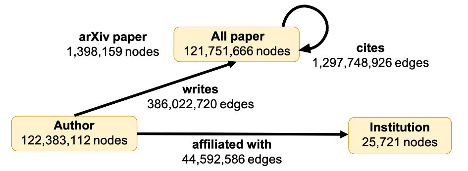
Example: MAG240M-LSC¶

The MAG240M-LSC graph is a heterogeneous academic graph extracted from the Microsoft Academic Graph (MAG), whose schema diagram is illustrated below:

https://data.dgl.ai/asset/image/guide_7_mag240m.png

Its raw data files are organized as follows:

/mydata/MAG240M-LSC/
  |-- meta.pt   # # A dictionary of the number of nodes for each type saved by torch.save,
  |             # as well as num_classes
  |-- processed/
    |-- author___affiliated_with___institution/
    |  |-- edge_index.npy            # graph, 713 MB
    |
    |-- paper/
    |  |-- node_feat.npy             # feature, 187 GB, (numpy memmap format)
    |  |-- node_label.npy            # label, 974 MB
    |  |-- node_year.npy             # year, 974 MB
    |
    |-- paper___cites___paper/
    |  |-- edge_index.npy            # graph, 21 GB
    |
    |-- author___writes___paper/
       |-- edge_index.npy            # graph, 6GB

The graph has three node types ("paper", "author" and "institution"), three edge types/relations ("cites", "writes" and "affiliated_with"). The "paper" nodes have three attributes ("feat", "label", "year"'), while other types of nodes and edges are featureless. Below shows the data files when it is stored in DGL Chunked Graph Format:

/mydata/MAG240M-LSC_chunked/
  |-- metadata.json            # metadata json file
  |-- edges/                   # stores edge ID data
  |  |-- writes-part1.csv
  |  |-- writes-part2.csv
  |  |-- affiliated_with-part1.csv
  |  |-- affiliated_with-part2.csv
  |  |-- cites-part1.csv
  |  |-- cites-part1.csv
  |
  |-- node_data/               # stores node feature data
     |-- paper-feat-part1.npy
     |-- paper-feat-part2.npy
     |-- paper-label-part1.npy
     |-- paper-label-part2.npy
     |-- paper-year-part1.npy
     |-- paper-year-part2.npy

All the data files are chunked into two parts, including the edges of each relation (e.g., writes, affiliates, cites) and node features. If the graph has edge features, they will be chunked into multiple files too. All ID data are stored in CSV (we will illustrate the contents soon) while node features are stored in numpy arrays.

The metadata.json stores all the metadata information such as file names and chunk sizes (e.g., number of nodes, number of edges).

{
   "graph_name" : "MAG240M-LSC",  # given graph name
   "node_type": ["author", "paper", "institution"],
   "num_nodes_per_chunk": [
       [61191556, 61191556],      # number of author nodes per chunk
       [61191553, 61191552],      # number of paper nodes per chunk
       [12861, 12860]             # number of institution nodes per chunk
   ],
   # The edge type name is a colon-joined string of source, edge, and destination type.
   "edge_type": [
       "author:writes:paper",
       "author:affiliated_with:institution",
       "paper:cites:paper"
   ],
   "num_edges_per_chunk": [
       [193011360, 193011360],    # number of author:writes:paper edges per chunk
       [22296293, 22296293],      # number of author:affiliated_with:institution edges per chunk
       [648874463, 648874463]     # number of paper:cites:paper edges per chunk
   ],
   "edges" : {
        "author:write:paper" : {  # edge type
             "format" : {"name": "csv", "delimiter": " "},
             # The list of paths. Can be relative or absolute.
             "data" : ["edges/writes-part1.csv", "edges/writes-part2.csv"]
        },
        "author:affiliated_with:institution" : {
             "format" : {"name": "csv", "delimiter": " "},
             "data" : ["edges/affiliated_with-part1.csv", "edges/affiliated_with-part2.csv"]
        },
        "author:affiliated_with:institution" : {
             "format" : {"name": "csv", "delimiter": " "},
             "data" : ["edges/cites-part1.csv", "edges/cites-part2.csv"]
        }
   },
   "node_data" : {
        "paper": {       # node type
             "feat": {   # feature key
                 "format": {"name": "numpy"},
                 "data": ["node_data/paper-feat-part1.npy", "node_data/paper-feat-part2.npy"]
             },
             "label": {   # feature key
                 "format": {"name": "numpy"},
                 "data": ["node_data/paper-label-part1.npy", "node_data/paper-label-part2.npy"]
             },
             "year": {   # feature key
                 "format": {"name": "numpy"},
                 "data": ["node_data/paper-year-part1.npy", "node_data/paper-year-part2.npy"]
             }
        }
   },
   "edge_data" : {}  # MAG240M-LSC does not have edge features
}

There are three parts in metadata.json:

Graph schema information and chunk sizes, e.g., "node_type" , "num_nodes_per_chunk", etc.
Edge index data under key "edges".
Node/edge feature data under keys "node_data" and "edge_data".

The edge index files contain edges in the form of node ID pairs:

# writes-part1.csv
0
1
20
29
1203
...

Specification¶

In general, a chunked graph data folder just needs a metadata.json and a bunch of data files. The folder structure in the MAG240M-LSC example is not a strict requirement as long as metadata.json contains valid file paths.

metadata.json top-level keys:

graph_name: String. Unique name used by dgl.distributed.DistGraph to load graph.
node_type: List of string. Node type names.
num_nodes_per_chunk: List of list of integer. For graphs with \(T\) node types stored in \(P\) chunks, the value contains \(T\) integer lists. Each list contains \(P\) integers, which specify the number of nodes in each chunk.
edge_type: List of string. Edge type names in the form of <source node type>:<relation>:<destination node type>.
num_edges_per_chunk: List of list of integer. For graphs with \(R\) edge types stored in \(P\) chunks, the value contains \(R\) integer lists. Each list contains \(P\) integers, which specify the number of edges in each chunk.
edges: Dict of ChunkFileSpec. Edge index files. Dictionary keys are edge type names in the form of <source node type>:<relation>:<destination node type>.
node_data: Dict of ChunkFileSpec. Data files that store node attributes. Dictionary keys are node type names.
edge_data: Dict of ChunkFileSpec. Data files that store edge attributes. Dictionary keys are edge type names in the form of <source node type>:<relation>:<destination node type>.

ChunkFileSpec has two keys:

format: File format. Depending on the format name, users can configure more details about how to parse each data file.
- "csv": CSV file. Use the delimiter key to specify delimiter in use.
- "numpy": NumPy array binary file created by numpy.save().
data: List of string. File path to each data chunk. Support absolute path.

Tips for making chunked graph data¶

Depending on the raw data, the implementation could include:

Construct graphs out of non-structured data such as texts or tabular data.
Augment or transform the input graph struture or features. E.g., adding reverse or self-loop edges, normalizing features, etc.
Chunk the input graph structure and features into multiple data files so that each one can fit in CPU RAM for subsequent preprocessing steps.

To avoid running into out-of-memory error, it is recommended to process graph structures and feature data separately. Processing one chunk at a time can also reduce the maximal runtime memory footprint. As an example, DGL provides a tools/chunk_graph.py script that chunks an in-memory feature-less DGLGraph and feature tensors stored in numpy.memmap.

Step.1 Graph Partitioning¶

This step reads the chunked graph data and calculates which partition each node should belong to. The results are saved in a set of partition assignment files. For example, to randomly partition MAG240M-LSC to two parts, run the partition_algo/random_partition.py script in the tools folder:

python /my/repo/dgl/tools/partition_algo/random_partition.py
    --in_dir /mydata/MAG240M-LSC_chunked
    --out_dir /mydata/MAG240M-LSC_2parts
    --num_partitions 2

, which outputs files as follows:

MAG240M-LSC_2parts/
  |-- paper.txt
  |-- author.txt
  |-- institution.txt

Each file stores the partition assignment of the corresponding node type. The contents are the partition ID of each node stored in lines, i.e., line i is the partition ID of node i.

# paper.txt
0
1
1
0
0
1
0
...

Note

DGL currently requires the number of data chunks and the number of partitions to be the same.

Despite its simplicity, random partitioning may result in frequent cross-machine communication. Check out chapter 7.4 Advanced Graph Partitioning for more advanced options.

Step.2 Data Dispatching¶

DGL provides a dispatch_data.py script to physically partition the data and dispatch partitions to each training machines. It will also convert the data once again to data objects that can be loaded by DGL training processes efficiently. The entire step can be further accelerated using multi-processing.

python /myrepo/dgl/tools/dispatch_data.py         \
   --in-dir /mydata/MAG240M-LSC_chunked/          \
   --partitions-dir /mydata/MAG240M-LSC_2parts/   \
   --out-dir data/MAG_LSC_partitioned            \
   --ip-config ip_config.txt

--in-dir specifies the path to the folder of the input chunked graph data produced
--partitions-dir specifies the path to the partition assignment folder produced by Step.1.
--out-dir specifies the path to stored the data partition on each machine.
--ip-config specifies the IP configuration file of the cluster.

An example IP configuration file is as follows:

172.31.19.1
172.31.23.205

During data dispatching, DGL assumes that the combined CPU RAM of the cluster is able to hold the entire graph data. Moreover, the number of machines (IPs) must be the same as the number of partitions. Node ownership is determined by the result of partitioning algorithm where as for edges the owner of the destination node also owns the edge as well.