6.4 Customizing Neighborhood Sampler
Although DGL provides some neighborhood sampling strategies, sometimes users would want to write their own sampling strategy. This section explains how to write your own strategy and plug it into your stochastic GNN training framework.
Recall that in How Powerful are Graph Neural Networks, the definition of message passing is:
where \(\rho^{(l)}\) and \(\phi^{(l)}\) are parameterized functions, and \(\mathcal{N}(v)\) is defined as the set of predecessors (or neighbors if the graph is undirected) of \(v\) on graph \(\mathcal{G}\).
For instance, to perform a message passing for updating the red node in the following graph:
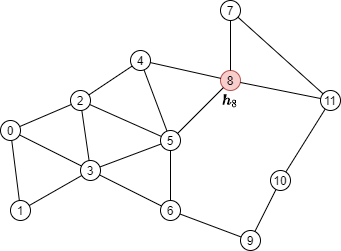
One needs to aggregate the node features of its neighbors, shown as green nodes:
Neighborhood sampling with pencil and paper
Let’s first define a DGL graph according to the above image.
import torch
import dgl

src = torch.LongTensor(
    [0, 0, 0, 1, 2, 2, 2, 3, 3, 4, 4, 5, 5, 6, 7, 7, 8, 9, 10,
     1, 2, 3, 3, 3, 4, 5, 5, 6, 5, 8, 6, 8, 9, 8, 11, 11, 10, 11])
dst = torch.LongTensor(
    [1, 2, 3, 3, 3, 4, 5, 5, 6, 5, 8, 6, 8, 9, 8, 11, 11, 10, 11,
     0, 0, 0, 1, 2, 2, 2, 3, 3, 4, 4, 5, 5, 6, 7, 7, 8, 9, 10])
g = dgl.graph((src, dst))
We then consider how multi-layer message passing works for computing the output of a single node. In the following text we refer to the nodes whose GNN outputs are to be computed as seed nodes.
Finding the message passing dependency
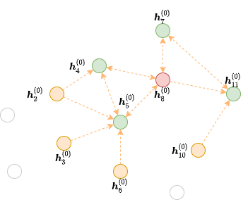
Consider computing with a 2-layer GNN the output of the seed node 8, colored red, in the following graph:

By the formulation:
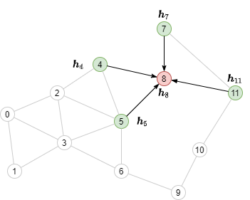
We can tell from the formulation that to compute \(\boldsymbol{h}_8^{(2)}\) we need messages from node 4, 5, 7 and 11 (colored green) along the edges visualized below.
This graph contains all the nodes in the original graph but only the edges necessary for message passing to the given output nodes. We call that the frontier of the second GNN layer for the red node 8.
Several functions can be used for generating frontiers. For instance,
dgl.in_subgraph() is a function that induces a
subgraph by including all the nodes in the original graph, but only all
the incoming edges of the given nodes. You can use that as a frontier
for message passing along all the incoming edges.
frontier = dgl.in_subgraph(g, [8])
print(frontier.all_edges())
For a concrete list, please refer to Subgraph Extraction Ops and dgl.sampling.
Technically, any graph that has the same set of nodes as the original graph can serve as a frontier. This serves as the basis for Implementing a Custom Neighbor Sampler.
The Bipartite Structure for Multi-layer Minibatch Message Passing
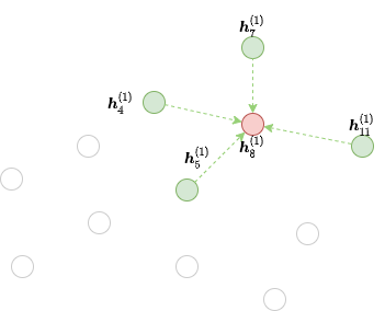
However, to compute \(\boldsymbol{h}_8^{(2)}\) from \(\boldsymbol{h}_\cdot^{(1)}\), we cannot simply perform message passing on the frontier directly, because it still contains all the nodes from the original graph. Namely, we only need nodes 4, 5, 7, 8, and 11 (green and red nodes) as input, as well as node 8 (red node) as output. Since the number of nodes for input and output is different, we need to perform message passing on a small, bipartite-structured graph instead. We call such a bipartite-structured graph that only contains the necessary input nodes (referred as source nodes) and output nodes (referred as destination nodes) of a message flow graph (MFG).
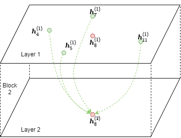
The following figure shows the MFG of the second GNN layer for node 8.
Note
See the Stochastic Training Tutorial for the concept of message flow graph.
Note that the destination nodes also appear in the source nodes. The reason is that representations of destination nodes from the previous layer are needed for feature combination after message passing (i.e. \(\phi^{(2)}\)).
DGL provides dgl.to_block() to convert any frontier
to a MFG where the first argument specifies the frontier and the
second argument specifies the destination nodes. For instance, the frontier
above can be converted to a MFG with destination node 8 with the code as
follows.
dst_nodes = torch.LongTensor([8])
block = dgl.to_block(frontier, dst_nodes)
To find the number of source nodes and destination nodes of a given node type,
one can use dgl.DGLHeteroGraph.number_of_src_nodes() and
dgl.DGLHeteroGraph.number_of_dst_nodes() methods.
num_src_nodes, num_dst_nodes = block.number_of_src_nodes(), block.number_of_dst_nodes()
print(num_src_nodes, num_dst_nodes)
The MFG’s source node features can be accessed via member
dgl.DGLHeteroGraph.srcdata and dgl.DGLHeteroGraph.srcnodes, and
its destination node features can be accessed via member
dgl.DGLHeteroGraph.dstdata and dgl.DGLHeteroGraph.dstnodes. The
syntax of srcdata/dstdata and srcnodes/dstnodes are
identical to dgl.DGLHeteroGraph.ndata and
dgl.DGLHeteroGraph.nodes in normal graphs.
block.srcdata['h'] = torch.randn(num_src_nodes, 5)
block.dstdata['h'] = torch.randn(num_dst_nodes, 5)
If a MFG is converted from a frontier, which is in turn converted from a graph, one can directly read the feature of the MFG’s source and destination nodes via
print(block.srcdata['x'])
print(block.dstdata['y'])
Note
The original node IDs of the source nodes and destination nodes in the MFG
can be found as the feature dgl.NID, and the mapping from the
MFG’s edge IDs to the input frontier’s edge IDs can be found as the
feature dgl.EID.
DGL ensures that the destination nodes of a MFG will always appear in the source nodes. The destination nodes will always index firstly in the source nodes.
src_nodes = block.srcdata[dgl.NID]
dst_nodes = block.dstdata[dgl.NID]
assert torch.equal(src_nodes[:len(dst_nodes)], dst_nodes)
As a result, the destination nodes must cover all nodes that are the destination of an edge in the frontier.
For example, consider the following frontier
where the red and green nodes (i.e. node 4, 5, 7, 8, and 11) are all nodes that is a destination of an edge. Then the following code will raise an error because the destination nodes did not cover all those nodes.
dgl.to_block(frontier2, torch.LongTensor([4, 5])) # ERROR
However, the destination nodes can have more nodes than above. In this case, we will have isolated nodes that do not have any edge connecting to it. The isolated nodes will be included in both source nodes and destination nodes.
# Node 3 is an isolated node that do not have any edge pointing to it.
block3 = dgl.to_block(frontier2, torch.LongTensor([4, 5, 7, 8, 11, 3]))
print(block3.srcdata[dgl.NID])
print(block3.dstdata[dgl.NID])
Heterogeneous Graphs
MFGs also work on heterogeneous graphs. Let’s say that we have the following frontier:
hetero_frontier = dgl.heterograph({
    ('user', 'follow', 'user'): ([1, 3, 7], [3, 6, 8]),
    ('user', 'play', 'game'): ([5, 5, 4], [6, 6, 2]),
    ('game', 'played-by', 'user'): ([2], [6])
}, num_nodes_dict={'user': 10, 'game': 10})
One can also create a MFG with destination nodes User #3, #6, and #8, as well as Game #2 and #6.
hetero_block = dgl.to_block(hetero_frontier, {'user': [3, 6, 8], 'game': [2, 6]})
One can also get the source nodes and destination nodes by type:
# source users and games
print(hetero_block.srcnodes['user'].data[dgl.NID], hetero_block.srcnodes['game'].data[dgl.NID])
# destination users and games
print(hetero_block.dstnodes['user'].data[dgl.NID], hetero_block.dstnodes['game'].data[dgl.NID])
Implementing a Custom Neighbor Sampler
Recall that the following code performs neighbor sampling for node classification.
sampler = dgl.dataloading.MultiLayerFullNeighborSampler(2)
To implement your own neighborhood sampling strategy, you basically
replace the sampler object with your own. To do that, let’s first
see what BlockSampler, the parent class of
MultiLayerFullNeighborSampler, is.
BlockSampler is responsible for
generating the list of MFGs starting from the last layer, with method
sample_blocks(). The default implementation of
sample_blocks is to iterate backwards, generating the frontiers and
converting them to MFGs.
Therefore, for neighborhood sampling, you only need to implement
thesample_frontier()method. Given which
layer the sampler is generating frontier for, as well as the original
graph and the nodes to compute representations, this method is
responsible for generating a frontier for them.
Meanwhile, you also need to pass how many GNN layers you have to the parent class.
For example, the implementation of
MultiLayerFullNeighborSampler can
go as follows.
class MultiLayerFullNeighborSampler(dgl.dataloading.BlockSampler):
    def __init__(self, n_layers):
        super().__init__(n_layers)

    def sample_frontier(self, block_id, g, seed_nodes):
        frontier = dgl.in_subgraph(g, seed_nodes)
        return frontier
dgl.dataloading.neighbor.MultiLayerNeighborSampler, a more
complicated neighbor sampler class that allows you to sample a small
number of neighbors to gather message for each node, goes as follows.
class MultiLayerNeighborSampler(dgl.dataloading.BlockSampler):
    def __init__(self, fanouts):
        super().__init__(len(fanouts))

        self.fanouts = fanouts

    def sample_frontier(self, block_id, g, seed_nodes):
        fanout = self.fanouts[block_id]
        if fanout is None:
            frontier = dgl.in_subgraph(g, seed_nodes)
        else:
            frontier = dgl.sampling.sample_neighbors(g, seed_nodes, fanout)
        return frontier
Although the functions above can generate a frontier, any graph that has the same nodes as the original graph can serve as a frontier.
For example, if one want to randomly drop inbound edges to the seed nodes with a probability, one can simply define the sampler as follows:
class MultiLayerDropoutSampler(dgl.dataloading.BlockSampler):
    def __init__(self, p, num_layers):
        super().__init__(num_layers)

        self.p = p

    def sample_frontier(self, block_id, g, seed_nodes, *args, **kwargs):
        # Get all inbound edges to `seed_nodes`
        src, dst = dgl.in_subgraph(g, seed_nodes).all_edges()
        # Randomly select edges with a probability of p
        mask = torch.zeros_like(src).bernoulli_(self.p)
        src = src[mask]
        dst = dst[mask]
        # Return a new graph with the same nodes as the original graph as a
        # frontier
        frontier = dgl.graph((src, dst), num_nodes=g.number_of_nodes())
        return frontier

    def __len__(self):
        return self.num_layers
After implementing your sampler, you can create a data loader that takes in your sampler and it will keep generating lists of MFGs while iterating over the seed nodes as usual.
sampler = MultiLayerDropoutSampler(0.5, 2)
dataloader = dgl.dataloading.NodeDataLoader(
    g, train_nids, sampler,
    batch_size=1024,
    shuffle=True,
    drop_last=False,
    num_workers=4)

model = StochasticTwoLayerRGCN(in_features, hidden_features, out_features)
model = model.cuda()
opt = torch.optim.Adam(model.parameters())

for input_nodes, blocks in dataloader:
    blocks = [b.to(torch.device('cuda')) for b in blocks]
    input_features = blocks[0].srcdata     # returns a dict
    output_labels = blocks[-1].dstdata     # returns a dict
    output_predictions = model(blocks, input_features)
    loss = compute_loss(output_labels, output_predictions)
    opt.zero_grad()
    loss.backward()
    opt.step()
Heterogeneous Graphs
Generating a frontier for a heterogeneous graph is nothing different
than that for a homogeneous graph. Just make the returned graph have the
same nodes as the original graph, and it should work fine. For example,
we can rewrite the MultiLayerDropoutSampler above to iterate over
all edge types, so that it can work on heterogeneous graphs as well.
class MultiLayerDropoutSampler(dgl.dataloading.BlockSampler):
    def __init__(self, p, num_layers):
        super().__init__(num_layers)

        self.p = p

    def sample_frontier(self, block_id, g, seed_nodes, *args, **kwargs):
        # Get all inbound edges to `seed_nodes`
        sg = dgl.in_subgraph(g, seed_nodes)

        new_edges_masks = {}
        # Iterate over all edge types
        for etype in sg.canonical_etypes:
            edge_mask = torch.zeros(sg.number_of_edges(etype))
            edge_mask.bernoulli_(self.p)
            new_edges_masks[etype] = edge_mask.bool()

        # Return a new graph with the same nodes as the original graph as a
        # frontier
        frontier = dgl.edge_subgraph(new_edges_masks, relabel_nodes=False)
        return frontier

    def __len__(self):
        return self.num_layers