5.4 Graph Classification
Instead of a big single graph, sometimes one might have the data in the form of multiple graphs, for example a list of different types of communities of people. By characterizing the friendship among people in the same community by a graph, one can get a list of graphs to classify. In this scenario, a graph classification model could help identify the type of the community, i.e. to classify each graph based on the structure and overall information.
Overview
The major difference between graph classification and node classification or link prediction is that the prediction result characterizes the property of the entire input graph. One can perform the message passing over nodes/edges just like the previous tasks, but also needs to retrieve a graph-level representation.
The graph classification pipeline proceeds as follows:
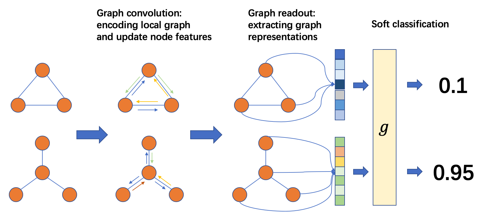
Graph Classification Process
From left to right, the common practice is:
Prepare a batch of graphs
Perform message passing on the batched graphs to update node/edge features
Aggregate node/edge features into graph-level representations
Classify graphs based on graph-level representations
Batch of Graphs
Usually a graph classification task trains on a lot of graphs, and it will be very inefficient to use only one graph at a time when training the model. Borrowing the idea of mini-batch training from common deep learning practice, one can build a batch of multiple graphs and send them together for one training iteration.
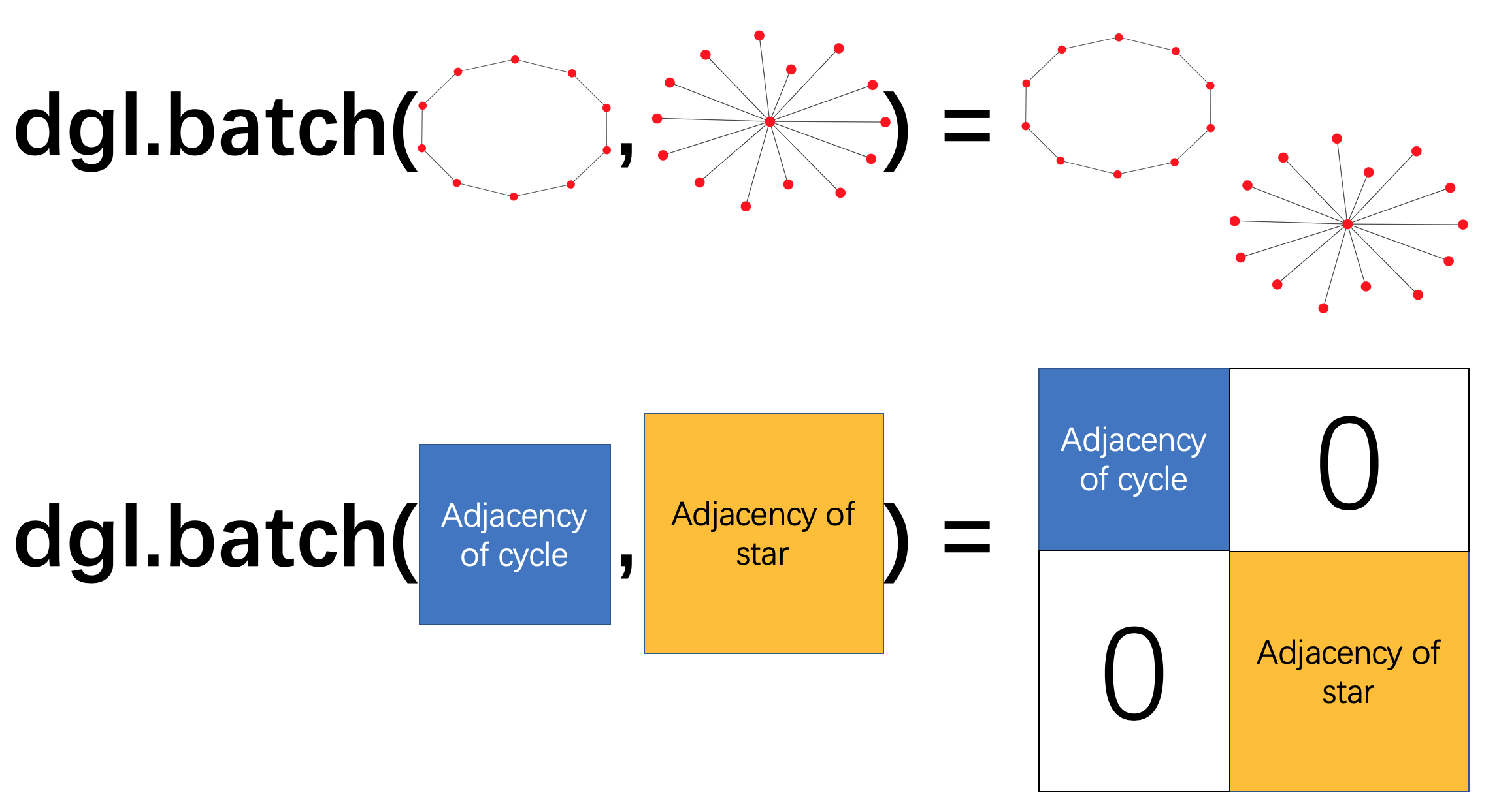
In DGL, one can build a single batched graph from a list of graphs. This batched graph can be simply used as a single large graph, with connected components corresponding to the original small graphs.
Batched Graph
The following example calls dgl.batch() on a list of graphs.
A batched graph is a single graph, while it also carries information
about the list.
import dgl
import torch as th

g1 = dgl.graph((th.tensor([0, 1, 2]), th.tensor([1, 2, 3])))
g2 = dgl.graph((th.tensor([0, 0, 0, 1]), th.tensor([0, 1, 2, 0])))

bg = dgl.batch([g1, g2])
bg
# Graph(num_nodes=7, num_edges=7,
#       ndata_schemes={}
#       edata_schemes={})
bg.batch_size
# 2
bg.batch_num_nodes()
# tensor([4, 3])
bg.batch_num_edges()
# tensor([3, 4])
bg.edges()
# (tensor([0, 1, 2, 4, 4, 4, 5], tensor([1, 2, 3, 4, 5, 6, 4]))
Please note that most dgl transformation functions will discard the batch information.
In order to maintain such information, please use dgl.DGLGraph.set_batch_num_nodes()
and dgl.DGLGraph.set_batch_num_edges() on the transformed graph.
Graph Readout
Every graph in the data may have its unique structure, as well as its node and edge features. In order to make a single prediction, one usually aggregates and summarizes over the possibly abundant information. This type of operation is named readout. Common readout operations include summation, average, maximum or minimum over all node or edge features.
Given a graph \(g\), one can define the average node feature readout as
where \(h_g\) is the representation of \(g\), \(\mathcal{V}\) is the set of nodes in \(g\), \(h_v\) is the feature of node \(v\).
DGL provides built-in support for common readout operations. For example,
dgl.mean_nodes() implements the above readout operation.
Once \(h_g\) is available, one can pass it through an MLP layer for classification output.
Writing Neural Network Model
The input to the model is the batched graph with node and edge features.
Computation on a Batched Graph
First, different graphs in a batch are entirely separated, i.e. no edges between any two graphs. With this nice property, all message passing functions still have the same results.
Second, the readout function on a batched graph will be conducted over each graph separately. Assuming the batch size is \(B\) and the feature to be aggregated has dimension \(D\), the shape of the readout result will be \((B, D)\).
import dgl
import torch

g1 = dgl.graph(([0, 1], [1, 0]))
g1.ndata['h'] = torch.tensor([1., 2.])
g2 = dgl.graph(([0, 1], [1, 2]))
g2.ndata['h'] = torch.tensor([1., 2., 3.])

dgl.readout_nodes(g1, 'h')
# tensor([3.])  # 1 + 2

bg = dgl.batch([g1, g2])
dgl.readout_nodes(bg, 'h')
# tensor([3., 6.])  # [1 + 2, 1 + 2 + 3]
Finally, each node/edge feature in a batched graph is obtained by concatenating the corresponding features from all graphs in order.
bg.ndata['h']
# tensor([1., 2., 1., 2., 3.])
Model Definition
Being aware of the above computation rules, one can define a model as follows.
import dgl.nn.pytorch as dglnn
import torch.nn as nn

class Classifier(nn.Module):
    def __init__(self, in_dim, hidden_dim, n_classes):
        super(Classifier, self).__init__()
        self.conv1 = dglnn.GraphConv(in_dim, hidden_dim)
        self.conv2 = dglnn.GraphConv(hidden_dim, hidden_dim)
        self.classify = nn.Linear(hidden_dim, n_classes)

    def forward(self, g, h):
        # Apply graph convolution and activation.
        h = F.relu(self.conv1(g, h))
        h = F.relu(self.conv2(g, h))
        with g.local_scope():
            g.ndata['h'] = h
            # Calculate graph representation by average readout.
            hg = dgl.mean_nodes(g, 'h')
            return self.classify(hg)
Training Loop
Data Loading
Once the model is defined, one can start training. Since graph classification deals with lots of relatively small graphs instead of a big single one, one can train efficiently on stochastic mini-batches of graphs, without the need to design sophisticated graph sampling algorithms.
Assuming that one have a graph classification dataset as introduced in Chapter 4: Graph Data Pipeline.
import dgl.data
dataset = dgl.data.GINDataset('MUTAG', False)
Each item in the graph classification dataset is a pair of a graph and its label. One can speed up the data loading process by taking advantage of the GraphDataLoader to iterate over the dataset of graphs in mini-batches.
from dgl.dataloading import GraphDataLoader
dataloader = GraphDataLoader(
    dataset,
    batch_size=1024,
    drop_last=False,
    shuffle=True)
Training loop then simply involves iterating over the dataloader and updating the model.
import torch.nn.functional as F

# Only an example, 7 is the input feature size
model = Classifier(7, 20, 5)
opt = torch.optim.Adam(model.parameters())
for epoch in range(20):
    for batched_graph, labels in dataloader:
        feats = batched_graph.ndata['attr']
        logits = model(batched_graph, feats)
        loss = F.cross_entropy(logits, labels)
        opt.zero_grad()
        loss.backward()
        opt.step()
For an end-to-end example of graph classification, see
DGL’s GIN example.
The training loop is inside the
function train in
main.py.
The model implementation is inside
gin.py
with more components such as using
dgl.nn.pytorch.GINConv (also available in MXNet and Tensorflow)
as the graph convolution layer, batch normalization, etc.
Heterogeneous graph
Graph classification with heterogeneous graphs is a little different from that with homogeneous graphs. In addition to graph convolution modules compatible with heterogeneous graphs, one also needs to aggregate over the nodes of different types in the readout function.
The following shows an example of summing up the average of node representations for each node type.
class RGCN(nn.Module):
    def __init__(self, in_feats, hid_feats, out_feats, rel_names):
        super().__init__()

        self.conv1 = dglnn.HeteroGraphConv({
            rel: dglnn.GraphConv(in_feats, hid_feats)
            for rel in rel_names}, aggregate='sum')
        self.conv2 = dglnn.HeteroGraphConv({
            rel: dglnn.GraphConv(hid_feats, out_feats)
            for rel in rel_names}, aggregate='sum')

    def forward(self, graph, inputs):
        # inputs is features of nodes
        h = self.conv1(graph, inputs)
        h = {k: F.relu(v) for k, v in h.items()}
        h = self.conv2(graph, h)
        return h

class HeteroClassifier(nn.Module):
    def __init__(self, in_dim, hidden_dim, n_classes, rel_names):
        super().__init__()

        self.rgcn = RGCN(in_dim, hidden_dim, hidden_dim, rel_names)
        self.classify = nn.Linear(hidden_dim, n_classes)

    def forward(self, g):
        h = g.ndata['feat']
        h = self.rgcn(g, h)
        with g.local_scope():
            g.ndata['h'] = h
            # Calculate graph representation by average readout.
            hg = 0
            for ntype in g.ntypes:
                hg = hg + dgl.mean_nodes(g, 'h', ntype=ntype)
            return self.classify(hg)
The rest of the code is not different from that for homogeneous graphs.
# etypes is the list of edge types as strings.
model = HeteroClassifier(10, 20, 5, etypes)
opt = torch.optim.Adam(model.parameters())
for epoch in range(20):
    for batched_graph, labels in dataloader:
        logits = model(batched_graph)
        loss = F.cross_entropy(logits, labels)
        opt.zero_grad()
        loss.backward()
        opt.step()